Generative models especially with the emerge of Generative Adversarial Networks (GANs) have become the spotlight of Deep Learning in recent years. They have many applications in the wild and sometimes they are just for fun. One fun application that I really liked, was the use of GAN to generate fake Sharingans (to read more about what Sharingan is please read this article). Inspired by that video and PyTorch’s DCGAN tutorial, in this post I’m going to show you how to generate sharingans step by step. You can download the PyTorch source code from here. I highly recommend downloading the full source code because here I only explain important steps in writing a DL model, things such as config files are not discussed here. To read more about project configuration see my Hyper-parameter Management article.

To train a model, you have to address three stages:

Gathering and loading data
Designing the architecture
Loss function and train loop

I structured my project directory as follows (if you like the structure, I created a template here):

 └── sharinGAN/ 
 │  └──── conf/ 
 │  │  └──── optimizer/ 
 │  │  │  └──── adam.yaml  
 │  │  ├──── config.yaml  
 │  │  ├──── dirs.yaml  
 │  │  ├──── models.yaml  
 │  │  └──── train.yaml  
 │  └──── model/ 
 │  │  ├──── data_loader.py  
 │  │  ├──── __init__.py  
 │  │  └──── net.py  
 │  └──── sharingan_pics/ 
 │  │  ├──── 0.jpeg  
 │  │  ├──── 10.jpeg  
 │  │  ├──── ...
 │  ├──── train.py  
 │  └──── utils.py   
 ├── README.md  
 └── requirements.txt

Gathering and Loading Data

The first thing that we need, in every problem that we are going to solve with deep learning, is data. I gathered some Sharingan pictures from google image search. It is a fairly easy task, you just need to search for the keyword sharingan and save the pictures in a folder. I named mine sharing_pics. So now, we have to write the data_loader.

To do so, first, we need to import the required libraries. We need pathlib to read image directories, PIL, Python imaging library (hence the name) to read images from the disk, PyTorch’s abstract Dataset module to write a class which handles concurrent reading and preprocessing for us, and finally for loading the config files we use a custom function that resides in utils.py file:

from omegaconf import OmegaConf


def get_conf(name: str):
    cfg = OmegaConf.load(f"{name}.yaml")
    return cfg

from pathlib import Path
from PIL import Image

import torch
from torch.utils.data import Dataset

from utils import get_conf


class SharinganDataset(Dataset):
    def __init__(self, transform) -> None:
        # get data directory
        data_dir = get_conf("conf/dirs").train_data
        # store filenames
        # Path().iterdir() returns a generator, convert it to list
        self.filenames = list(Path(data_dir).iterdir())
        self.transform = transform

    def __len__(self) -> int:
        """return size of dataset"""
        return len(self.filenames)

    def __getitem__(self, idx) -> torch.tensor:
        # load the image
        image = Image.open(self.filenames[idx])
        # apply transformers on it and return it
        image = self.transform(image)
        return image

In SharinganDataset we read image addresses and store them in self.filenames. Our dataset size is the length of self.filenames, which in our case is 100. Every image that we want to read, it’s address is in self.filenames, we read the image with the help of PIL and then apply image transformations on it. Finally, the image is in the form that we want. In the train loop section, we will discuss these transformations. And that’s it for loading data.

Designing the Architecture

For the generator and discriminator architecture, we follow the DCGAN architecture and implement it as described in pytorch tutorial with one exception that BatchNorm2d is applied after the activation function. The code for model architectures resides in model/net.py. The noticeable network components here are:

ConvTranspose2d(in_channels, out_channels, kernel_size, stride, padding, bias): sometimes called deconvolution operator. But they are actually not the same. ConvTranspose applies filter on the spaced out (with zeros) input. The end result would be an upsampled of the input with learned weights. You can read more about it here with corresponding repo. The output height can be calculated with: $H_{out} =(H_{in} −1) \times stride[0]−2\times padding[0]+dilation[0]\times (kernel_size[0]−1)+outputpadding[0]+1$ and for the width: $W_{out} =(W_{in}−1) \times stride[1]−2\times padding[1]+dilation[1]\times (kernel_size[1]−1)+outputpadding[1]+1$
ReLU(inplace): as the activation function which is $max(0, x)$, and inplace is for doing the operation in-place in the output without using extra memory.
BatchNorm2d(num_features): which applies batch normalization on the input feature maps. You can read more about it here.
Conv2d(in_channels, out_channels, kernel_size, stride, padding, bias): is the convolution module.
LeakyRelU(negative_slope, inplace): is a derivative of ReLU which is not strictly hard on negative values. negative_slope is responsible for this softness.
Sigmoid(): an activation function which squashed the output to be between $[0, 1]$ just like a probability.

import torch.nn as nn

from utils import get_conf


class Generator(nn.Module):
    def __init__(self):
        super(Generator, self).__init__()
        self.cfg = get_conf("conf/model/generator")

        self.gen = nn.Sequential(
            # input is Z, going into a convolution
            nn.ConvTranspose2d(
                self.cfg.nz, self.cfg.ngf * 8, 4, 1, 0, 
                bias=False),
            nn.ReLU(True),
            nn.BatchNorm2d(self.cfg.ngf * 8),
            # state size. (ngf*8) x 4 x 4
            nn.ConvTranspose2d(
                self.cfg.ngf * 8, self.cfg.ngf * 4, 4, 2, 1, 
                bias=False),
            nn.ReLU(True),
            nn.BatchNorm2d(self.cfg.ngf * 4),
            # state size. (ngf*4) x 8 x 8
            nn.ConvTranspose2d(
                self.cfg.ngf * 4, self.cfg.ngf * 2, 4, 2, 1, 
                bias=False),
            nn.ReLU(True),
            nn.BatchNorm2d(self.cfg.ngf * 2),
            # state size. (ngf*2) x 16 x 16
            nn.ConvTranspose2d(
                self.cfg.ngf * 2, self.cfg.ngf, 4, 2, 1, 
                bias=False),
            nn.ReLU(True),
            nn.BatchNorm2d(self.cfg.ngf),
            # state size. (ngf) x 32 x 32
            nn.ConvTranspose2d(
                self.cfg.ngf, self.cfg.nc, 4, 2, 1, 
                bias=False),
            nn.Tanh()
            # state size. (nc) x 64 x 64
        )

    def forward(self, input):
        return self.gen(input)


class Discriminator(nn.Module):
    def __init__(self):
        super(Discriminator, self).__init__()
        self.cfg = get_conf("conf/model/discriminator")

        self.dis = nn.Sequential(
            # input is (nc) x 64 x 64
            nn.Conv2d(
                self.cfg.nc, self.cfg.ndf, 4, 2, 1, 
                bias=False),
            nn.LeakyReLU(0.2, inplace=True),
            # state size. (ndf) x 32 x 32
            nn.Conv2d(
                self.cfg.ndf, self.cfg.ndf * 2, 4, 2, 1, 
                bias=False),
            nn.LeakyReLU(0.2, inplace=True),
            nn.BatchNorm2d(self.cfg.ndf * 2),
            # state size. (ndf*2) x 16 x 16
            nn.Conv2d(
                self.cfg.ndf * 2, self.cfg.ndf * 4, 4, 2, 1, 
                bias=False),
            nn.LeakyReLU(0.2, inplace=True),
            nn.BatchNorm2d(self.cfg.ndf * 4),
            # state size. (ndf*4) x 8 x 8
            nn.Conv2d(
                self.cfg.ndf * 4, self.cfg.ndf * 8, 4, 2, 1, 
                bias=False),
            nn.LeakyReLU(0.2, inplace=True),
            nn.BatchNorm2d(self.cfg.ndf * 8),
            # state size. (ndf*8) x 4 x 4
            nn.Conv2d(
                self.cfg.ndf * 8, 1, 4, 1, 0, 
                bias=False),
            nn.Sigmoid()
        )

    def forward(self, input):
        return self.dis(input)

The generator (from now on we call it G) is responsible for generating images like real Sharingans. Therefore, it’s output must be an image with the same size as the real images ((3, 64, 64) tensors). On the other side, the discriminator (D) is responsible to decide the authenticity of input images, it outputs 1 where the image is real and 0 where it is fake. Actually, the discriminator is not that accurate, it outputs the probability of the image being authentic. Where close to 1 means the discriminator is somewhat sure that the image is real and close to 0 means vice versa. That’s why we need a Sigmoid() function at the end of the discriminator. This takes us to the last part of this project which is defining the loss function and training loop.

Loss function and Train loop

GANs train a little different from normal networks. It is a zero-sum game between two networks where one tries to fool another to accept its outputs as authentic. The loss function, defined to do so, is called adversarial loss:

\[min_G max_D log(D(x))+log(1−D(G(z)))\]

You can read more about it in the original paper:

This is very similar to binary cross-entropy where we have:

\[ylog(x)+(1-y)log(1−x)\]

Training GANs is very tricky, I suggest reading GAN hacks page which contains useful information regarding training GANs. We split training into two parts, one for the discriminator and one for the generator.

Training Discriminator

The sole purpose of the discriminator is to classify real and fake images with high probability. Which means we want to maximize $log(D(x))+log(1−D(G(z)))$ According to GAN hacks, we use two batches, one batch for true images and one for fake images. After forward pass of real images we label of 1, we perform one backward() pass to calculate derivatives, then we pass fake (generated) images to D with label of 0 and perform another backward() pass to accumulate gradients and then update the weights.

Training Generator

According to original paper G wants to minimize $log(1−D(G(z)))$ Minimizing this means fooling D to output high probability (1 means they are real) therefor this part will descend to 0. But in the early stages of training, this is very unlikely that the D discriminates well, as a result of this, G won’t get better. But instead maximizing $log(D(G(z)))$ would solve this issue. To only use $log(D(G(z)))$ part of binary cross-entropy we need to pass the label 1 with G outputs to the discriminator.

That’s it. There are just little modifications left in order to start the training. According to GAN hacks, initializing weights with normal distribution yield better results. To do so, we need a function to do this for us:

def init_weights(m):
    # get the module name
    classname = m.__class__.__name__
    # if it is in ['Conv', 'BatchNorm', 'Linear'], apply normal initialization
    if classname.find('Conv') != -1:
        nn.init.normal_(m.weight.data, 0.0, 0.02)
    elif classname.find('BatchNorm') != -1:
        nn.init.normal_(m.weight.data, 1.0, 0.02)
        nn.init.constant_(m.bias.data, 0)
    elif classname.find('Linear') != -1:
        nn.init.normal_(m.weight.data, 1.0, 0.02)
        nn.init.constant_(m.bias.data, 0)

And here is the training loop, some functions are imported from utils.py that you can find in the source code:

import numpy as np
import torch
from torchvision import transforms
import torchvision.utils as vutils
from torch.utils.data import DataLoader
import torch.nn as nn
import torch.optim as optim
import matplotlib.pyplot as plt

from utils import get_device, plot_images, weights_init, get_conf
from model.data_loader import SharinganDataset
from model.net import Discriminator, Generator


def main():
    cfg = get_conf("conf/train")
    device = get_device()
    # Create the generator
    netG = Generator().to(device)

    # Handle multi-gpu
    if (device.type == 'cuda') and (cfg.ngpu > 1):
        netG = nn.DataParallel(netG, list(range(cfg.ngpu)))

    # Apply the weights_init function to randomly
    # initialize all weights to mean=0, stdev=0.2.
    netG.apply(init_weights)
    # Create the Discriminator
    netD = Discriminator().to(device)

    # Handle multi-gpu if desired
    if (device.type == 'cuda') and (cfg.ngpu > 1):
        netD = nn.DataParallel(netD, list(range(cfg.ngpu)))

    # Apply the weights_init function to randomly
    # initialize all weights to mean=0, stdev=0.2.
    netD.apply(init_weights)
    # transform images: 
    # Resize to 64x64 -> Center crop -> Convert to tensor-> normalize
    transform = transforms.Compose([
        transforms.Resize(cfg.image_size),
        transforms.CenterCrop(cfg.image_size),
        transforms.ToTensor(),
        transforms.Normalize((0.5, 0.5, 0.5), (0.5, 0.5, 0.5)),
    ])

    dataset = SharinganDataset(transform)
    dataloader = DataLoader(dataset, 
                            batch_size=cfg.batch_size,
                            shuffle=True, 
                            num_workers=cfg.workers)

    # Initialize BCELoss function
    criterion = nn.BCELoss()

    # Establish convention for real and fake labels during training
    fixed_noise = torch.randn(cfg.batch_size, 
                              cfg.nz, 1, 1, device=device)
    real_label = 1.
    fake_label = 0.
    # load adam optimizer's config
    cfg_adam = get_conf("conf/optimizer/adam")
    # Setup Adam optimizers for both G and D
    optimizerD = optim.Adam(netD.parameters(), 
                            lr=cfg_adam.lr, 
                            betas=(cfg_adam.beta1, 0.999))
    optimizerG = optim.Adam(netG.parameters(), 
                            lr=cfg_adam.lr, 
                            betas=(cfg_adam.beta1, 0.999))
    # Training Loop

    # Lists to keep track of progress
    img_list = []
    G_losses = []
    D_losses = []
    iters = 0

    print("Starting Training Loop...")
    # For each epoch
    for epoch in range(cfg.num_epochs):
        # For each batch in the dataloader
        for i, data in enumerate(dataloader, 0):

            ############################
            # (1) Update D network: 
            # maximize log(D(x)) + log(1 - D(G(z)))
            ###########################
            ## Train with all-real batch
            netD.zero_grad()
            # send data batch to the device
            real_cpu = data.to(device)
            # get batch size
            b_size = real_cpu.size(0)
            # create labels for real images, 
            # we need labels for each image in the batch
            label = torch.full((b_size,), 
                               real_label, 
                               dtype=torch.float, 
                               device=device)
            # Forward pass real batch through D
            output = netD(real_cpu).view(-1)
            # Calculate loss on all-real batch
            errD_real = criterion(output, label)
            # Calculate gradients of real batch for D in backward pass
            errD_real.backward()
            D_x = output.mean().item()

            ## Train with all-fake batch
            # Generate batch of latent vectors
            noise = torch.randn(b_size, 
                                cfg.nz, 1, 1, device=device)
            # Generate fake image batch with G
            fake = netG(noise)
            label.fill_(fake_label)
            # Classify all fake batch with D
            # we need to detch the computation graph here
            # because we don't want update G here
            output = netD(fake.detach()).view(-1)
            # Calculate D's loss on the all-fake batch
            errD_fake = criterion(output, label)
            # Calculate the gradients of fake batch
            # for this batch (this gets accumulated)
            errD_fake.backward()
            D_G_z1 = output.mean().item()
            # Add the gradients from the all-real and
            # all-fake batches (just for visualization)
            errD = errD_real + errD_fake
            # Update D
            optimizerD.step()

            ############################
            # (2) Update G network: maximize log(D(G(z)))
            ###########################
            netG.zero_grad()
            label.fill_(real_label)  # fake labels are real for generator cost
            # Since we just updated D, perform another
            # forward pass of all-fake batch through D
            output = netD(fake).view(-1)
            # Calculate G's loss based on this output
            errG = criterion(output, label)
            # Calculate gradients for G
            errG.backward()
            D_G_z2 = output.mean().item()
            # Update G
            optimizerG.step()

            # Output training stats
            if i % 25 == 0:
                print('[%d/%d][%d/%d]\tLoss_D: %.4f\tLoss_G: %.4f\tD(x): %.4f\tD(G(z)): %.4f / %.4f'
                      % (epoch, cfg.num_epochs, i, len(dataloader),
                         errD.item(), errG.item(), D_x, D_G_z1, D_G_z2))

            # Save Losses for plotting later
            G_losses.append(errG.item())
            D_losses.append(errD.item())

            # Check how the generator is doing by
            # saving G's output on fixed_noise
            if (iters % 100 == 0) or ((epoch == cfg.num_epochs - 1) and (i == len(dataloader) - 1)):
                with torch.no_grad():
                    fake = netG(fixed_noise).detach().cpu()
                img_list.append(vutils.make_grid(fake, padding=2, normalize=True))

            iters += 1

This is like normal training but with a little adjustment where we need to train both D and G.

Results

After 200 epochs the results are like this:

As you can see, the generator learns some patterns from the data. Of course, if you train it for more epochs, it gets better and better. One improvement (again according to GAN hacks) that we can add is to train D more than G. The notion behind it is that if D do its job perfectly, then G challenged and need to can change more to keep up.

I perform another modification on D’s loss. As the output of D is a probability, its gradients are small, as a result, the changes in weights will be minor. To make gradients bigger for bigger changes, I add squared distance of real images with fake images to the D’s loss with some weight $\beta$ (here $\beta=0.01$). So, the D’s loss becomes this:

errD_fake = criterion(output, label) + (beta * (fake.detach() - real_cpu).pow(2).mean(0).sum())

Although we should keep this in mind, the gradients should not get too big. In the next section, I will discuss how to prevent this. But for now, this modification yields this result for 1000 epochs:

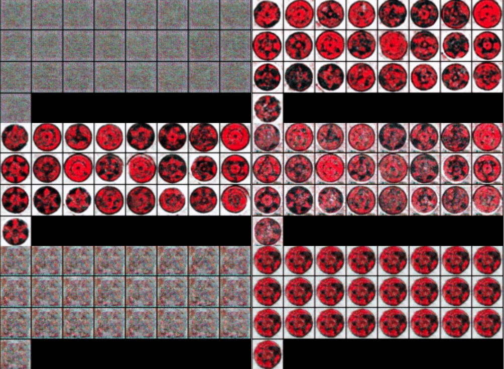
As you can see here, the images getting better and better until they hit a wall and reset, and at the end, G only generate one Sharingan, that is because this pattern was able to fool D and G does not bother itself to generate another Sharingan. This situation is called mode collapse in GAN literature.

If we take a look at the loss functions of D and G, we can see two spikes in D’s loss. Those spikes are exactly where we see that generated images falling apart. G generates garbage and D can’t decide.

Back to where we need to prevent gradients from exploding. To prevent this, we can add gradient clipping in order to prevent the gradients going higher than a threshold. One option is to use gradient clipping (here clipping_threshold_d = 5) which should be added just before updating weights:

if clipping_threshold_d > 0:
                    nn.utils.clip_grad_norm_(netD.parameters(),
                                     clipping_threshold_d)
# Update D
optimizerD.step()

Another option is to add spectral normalization to D to stabilize its training. I also added it to the G as well. To add this in code, when defining G and D components, instead of ConvTranspose2d and Conv2d add these:

nn.utils.spectral_norm(nn.ConvTranspose2d(...))
nn.utils.spectral_norm(nn.Conv2d(...))

With these optimizations and without modified D’s loss, after 200 epochs we get:

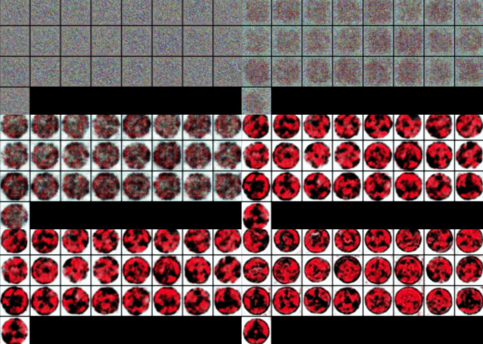
Comparing the first run with the optimized version, we can see that in the latter, G does its best to generate Sharingans with different patterns. After 800 more epochs:

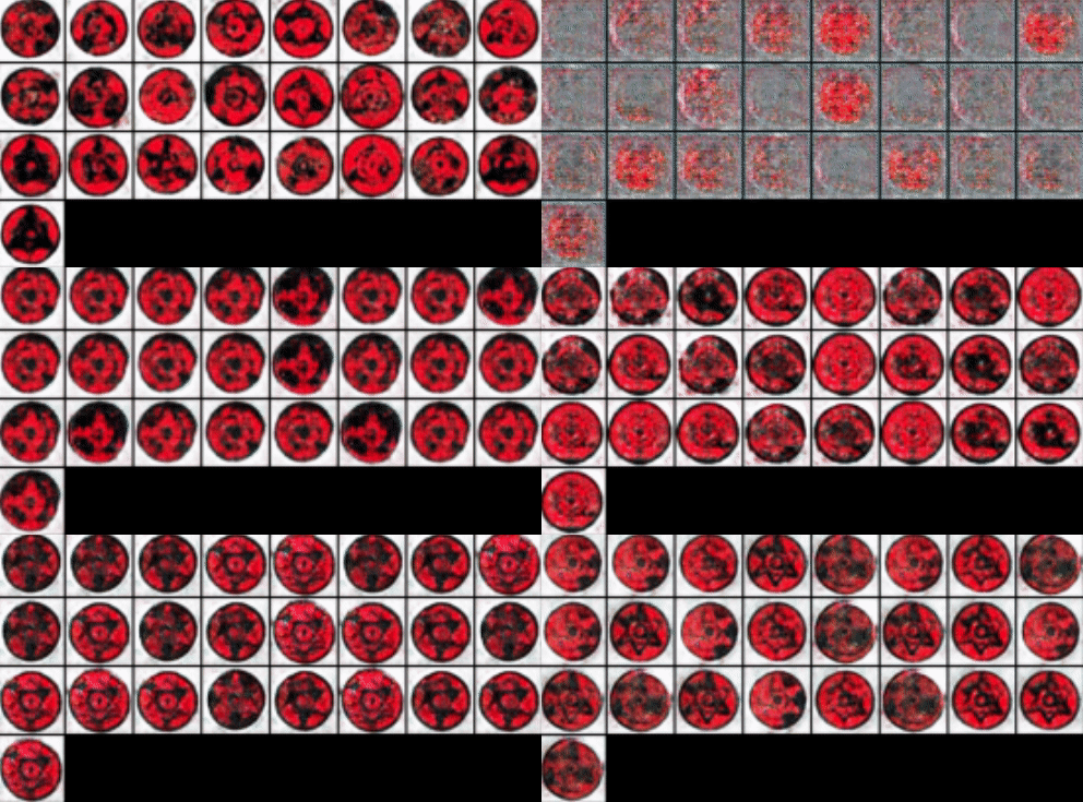
G collapsed again but this time it has more variety.

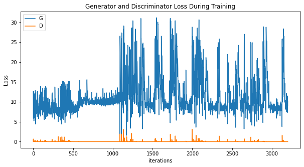
Taking a look at the loss function we can see this time we’ve managed to prevent spikes in D’s loss. If we train the model with fewer epochs the collapse would not occur. So 1000 epochs are overkill for this small dataset as in early epochs we can see good results and we should stop the training there (early stopping).

And here is the result with optimizations and modified D loss function after 300 epochs (I didn’t train it more because as we saw above, it is likely would collapse):

And for the loss:

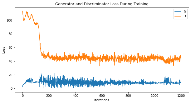
The loss is much better and more stable.

To be honest, with these low res images finding subtle patterns is difficult and G is doing a great job. For generating crystal clear Sharingan images we need improved derivatives of GAN. Hopefully, in future posts, I will talk about implementing them. And that’s it, I hope you enjoyed this post.

SharinGAN